We are going to demonstrate the maths behind a Support Vector Machine classifier.

Prerequisites: You should have a good grasp over linear algebra and basic understanding of supervised machine learning.

Support Vector Machines(SVMs) are one of the widely used binary classification algorithms in Machine Learning. SVMs works by maximizing margin. Let’s look at the Fig 1. for understanding how margin works.

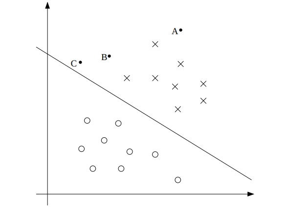Fig. 1: Margin in a typical binary classification problem

Fig. 1 represents a binary classification problem and the classes are linearly separable. If we take a point, A for example, the vertical distance between point A and the separating line represents the margin of point A w.r.t. the separating line. Now, intuitively the margin distance should reflect the confidence in class prediction as we move away from the separating line. Also the confidence in predicting C will be far less than that of A(and out margin should reflect that accordingly). We also notice that moving the separating line even a little may result in a wrong prediction for C. So, we would also like the separating hyperplane to be as far as possible from C, the closest point in among the ‘upper’ side of separating line.

Now let’s formulate the equation of the separating hyperplane based on the criterion described above. Now, we have the separating hyperplane L as shown in Fig. 2. We will work with the vector form of the equation:

\begin{equation} w^T*x + b = 0 \end{equation}

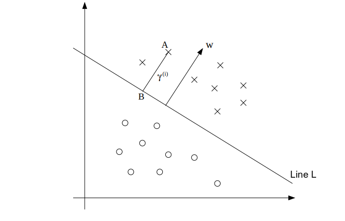Fig. 2: Margin and separating hyperplane in SVM binary classification.

If you are wondering why the w vector is perpendicular to separating line L, try to take an equation of a straight line and work it out. We can try to calculate the margin for point A as:

\begin{equation} \gamma^ \left( i \right) = length(AB) \end{equation}

Now, point A represents $x^{(i)}$ and hence we can write vector point B as the following:

\begin{equation} x^ \left( i \right) - \gamma^ \left( i \right) \frac {w}{||w||} \end{equation}

Since point B is on the separating line, it will satisfy $w^T*x + b=0$

\begin{equation} w^T \left( x^ \left( i \right) - \gamma^ \left( i \right) \frac {w}{||w||} \right) + b = 0 \end{equation}

Solving for $\gamma^{\left(i \right)}$:

\begin{equation} \gamma^ \left(i \right) \frac {w^T*w}{||w||} = w^Tx^{(i)} + b \end{equation}

Further, we can use the following to simplify the above equation \begin{equation} w^T\cdot w = {\left\lVert w \right\lVert}^2 \end{equation}

\begin{equation} \gamma^ \left(i \right) = \frac {w^Tx^ \left( i \right)+ b}{||w||} \end{equation}

Also, we note that for points above the separating line($y^{(i)} =1$), $w^{T}\cdot x+b >0$ (“positive” points) and for points below the separating line($y^{(i)}=-1$), $w^{T}\cdot x+b<0$ (“negative” points). We can modify the margin for a data point $x^ {(i)}, y^ {(i)}$ as following:

\begin{equation} \gamma^ \left(i \right) = y^ \left( i \right) \left(\frac{w^Tx^ \left(i \right) + b}{||w||}\right) \end{equation}

Now, there is something special about the margin we have obtained. if we change (w,b) to (2w,2b), the margin doesn’t change at all. Which means we can put some scaling constraint on (w,b) and still maintain the same margin for each point. We will use this later. We can now obtain the smallest margin given our data-set $x^ {(i)}, y^ {(i)}$ for $i \in (1,….,m)$ as the following:

\begin{equation} \gamma = \min_{i=1,….,m} \gamma^ \left(i \right) \end{equation}

Now that we have a nice form for the margin, we can formulate our optimization problem as below:

\begin{equation} \max_{w,b} \gamma \end{equation} \begin{equation} s.t. \left[ y^ \left( i \right) \left( \frac {w^Tx^ \left( i \right) + b}{||w||} \right) \right] \geq \gamma, i=1,….,m \end{equation}

The closest points from the separating hyperplane on both sides are called Support Vectors.

Now, as discussed above, we are free to put a scaling constraint on $(w,b)$. We will put the following constraint: \begin{equation} w^Tx + b = +1, \text{for the line going through support vector in the upper side} \end{equation} \begin{equation} w^Tx + b = -1, \text{for the line going through support vector in the lower side} \end{equation} Again, We are free to do this as this won’t affect our margin and just rescale $(w,b)$ accordingly. Also note that we are just putting a single constraint ($w^Tx + b = +1$) for the closest point on the upper side. The second constraint just follows the first one as the closest point should be same distance apart on both side of the separating hyperplane.

If you are still confused about the scaling constraint, let’s consider the equations going through the support vectors are $w_{1}^Tx + b_{1} = +c$ and $w_{1}^Tx + b_{1} = -c$ as shown in Fig. 3. Now, the equation of the separating hyperplane is $w_{1}^Tx + b_{1} = 0$. Now we can rewrite the equations as following:

\begin{equation} \frac {w_{1}^T}{c}x + \frac {b_{1}}{c} = 1 \end{equation} The second equation can be rewritten as the following: \begin{equation} \frac {w_{1}^T}{c}x + \frac {b_{1}}{c} = -1 \end{equation} And now the equation of the separating plane \begin{equation} \frac {w_{1}^T}{c}x + \frac {b_{1}}{c} = 0 \end{equation}

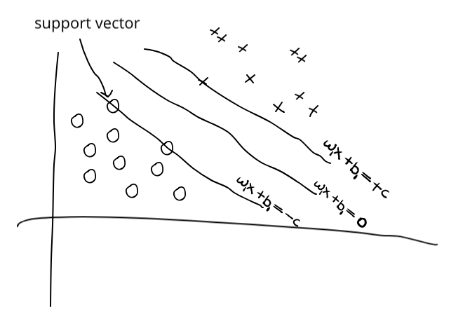Fig. 3: Support vectors.

If we take $w = \frac {w_{1}}{c}$ and $b = \frac {b_{1}}{c}$ the above equation becomes the following: \begin{equation} w^Tx + b = 1 \end{equation} \begin{equation} w^Tx + b = -1 \end{equation} \begin{equation} w^Tx + b = 0 \end{equation}

As you can see that the equation of the separating hyperplane hasn’t changed even if we take new $w^T = \frac {w_{1}^T}{c}$ and new $b = \frac {b_{1}}{c}$. The distance of the points are from separating are also not changing(we have already seen that). You can assume that the possible solutions for $(w,b,c)$ can be $(w,b,c)$, $(\frac {w}{c},\frac {b}{c},1)$ or even $(\frac {w}{2c},\frac {b}{2c}, \frac {1}{2})$. It just doesn’t make any difference as they all lead to the same solution.

Let’s use this for evaluating $\gamma$

\begin{equation} \gamma = \min_{i=1,….,m} \gamma^ \left(i \right) \end{equation}

\begin{equation} \gamma = \min_{i=1,….,m} \left[ y^ \left(i \right) \left( \frac {w^Tx^ {(i)} + b}{||w||} \right) \right] \end{equation}

\begin{equation} \gamma = \frac {1}{||w||} \end{equation}

This comes as $ y^ {(i)}=1 $ for the closest point on the upper side.

We can rewrite the optimization task as:

\begin{equation} \max_{w,b} \frac {1}{||w||} \end{equation} \begin{equation} or \min ||w|| \end{equation} \begin{equation} or \min \frac{1}{2} ||w||^2 \end{equation}

\begin{equation} s.t. \left[ y^ \left(i \right) (w^Tx^ \left(i \right)) + b ) \right] \geq 1, i=1,….,m \end{equation}

To incorporate the inequality in our optimization task, we can penalize the data-points with incorrect prediction. For example, in Fig. 1, if point C is getting predicted at the lower half of the separating line, we have a wrong prediction and we need to penalize the prediction to move the separating line(or hyperplane in general). For point C, if $ w^Tx^ {(i)} + b > 0$, then we need not penalize the data point, or the $ penalty = 0 $, but if $ w^Tx^ {(i)} + b < 0$, we can define the $ penalty = - \left( w^Tx^ {(i)} + b\right)$.

Now, we not only want the predictions to be on upper side for point C, but be far from the separating line. For this, we apply a condition that the prediction should be beyond the closest point from the separating line (i.e. For C, beyond $ w^Tx^ {(i)} + b = +1$). So, we can redefine the penalty as $ 1 - \left( w^Tx^ {(i)} + b \right) $. Our new optimization task becomes the following: \begin{equation} \min_{w,b} \left[ \frac {1}{2} ||w||^2 + \sum_{i=1}^{m} \max \left( 0, \left( 1 - \left( w^Tx^ \left(i \right) + b\right) \right) \right) \right] \end{equation}

This is what is called a Hard Margin Classifier as we are not allowing any of our data-points to be predicted incorrectly. Now there can be cases where we are dealing with some outliers and outlier data-points can influence our separating plane in an undesirable way. In the next problem we will allow some data-points to be predicted incorrectly. This is called a Soft Margin Classifier. I will incorporate the optimization task for Soft Margin Classifier in the coming days.

Future work:

1. Soft Margin Classifier
2. Optimization methods used for SVM
3. Using SVM where classes are not linearly separable
4. What are the attributes for an optimal data-set for SVM classifier
5. Why normalization is necessary in SVM